Data Visualization Roadmap (with Python)

Data Visualization: What it is , Why it’s so Important & How to Use It :

Data visualization is the graphical representation of information and data. By using visual elements like charts, graphs, and maps, data visualization tools provide an accessible way to see and understand trends, outliers, and patterns in data.

Why its so important ? Data visualization provides a quick and effective way to communicate information in a universal manner using visual information. The practice can also help businesses identify which factors affect customer behavior; pinpoint areas that need to be improved or need more attention; make data more memorable for stakeholders , understand when and where to place specific products; and predict sales volumes.

With the Pandas, Seaborn and Matplotlib we can easily plot different types of charts, graphs and maps.

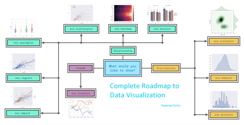
Let us break the chart types into three broad categories : –

Trends :- A trend is defined as a pattern of change.
sns.lineplot – Line charts are best to show trends over a period of time, and multiple lines can be used to show trends in more than one group.

Relationship :- There are many different chart types that you can use to understand relationships between variables in your data.
sns.barplot – Bar charts are useful for comparing quantities corresponding to different groups.
sns.heatmap – Heatmaps can be used to find color-coded patterns in tables of numbers.
sns.scatterplot – Scatter plots show the relationship between two continuous variables; if color-coded, we can also show the relationship with a third categorical variable.
sns.regplot – Including a regression line in the scatter plot makes it easier to see any linear relationship between two variables.
sns.lmplot – This command is useful for drawing multiple regression lines, if the scatter plot contains multiple, color-coded groups.
sns.swarmplot – Categorical scatter plots show the relationship between a continuous variable and a categorical variable

Distribution – We visualize distributions to show the possible values that we can expect to see in a variable, along with how likely they are.
sns.distplot – Histograms show the distribution of a single numerical variable.
sns.kdeplot – Kernal Density Estimate KDE plot (or 2D KDE plots) show an estimated, smooth distribution of a single numerical variable (or two numerical variables).
sns.jointplot – This command is useful for simultaneously displaying a 2D KDE plot with the corresponding KDE plots for each individual variable.

import pandas as pd
import matplotlib.pyplot as plt                 # importing modules
import seaborn as sns

file_path = "C:/...input/mydata.csv"    # CSV filepath  #to do
file_data = pd.read_csv(file_path, index_col = "SNo")   # read the csv file

file_data = file_data.head()   #-------> gives us the first 5 rows(default)
file_data = file_data.head(n)   #-------> gives us the first n rows

file_data = file_data.tail()   #-------> gives us the last 5 rows(default)
file_data = file_data.tail(n)  #-------> gives us the last n rows
print(file_data) 

plt.figure(figsize=(8,6))  #plt window

sns.set_style("dark")        #------> for dark theme

    ''' Available themes are.....
            "darkgrid"
            "whitegrid"
            "dark"
            "white"
            "ticks"
    '''

#LinePlot ->
sns.lineplot(data = file_data)

#BarPlot ->
sns.barplot(x=file_data.index , y=file_data["column_name"])

#Heatmap ->
sns.heatmap(data = file_data , annot = True)
                                                # Annot=True put the values in the cells
                        
#ScatterPlot ->
sns.scatterplot(x = file_data["column_name"], y =file_data["column_name"], hue = file_data["column_name"])
                                                # hue gives the color code
                                                
#RegPlot ->
sns.regplot(x=file_data["column_name"], y=file_data["column_name"])
                                                # Regression Line Plot

#Lmplot ->
sns.lmplot(x="column_name", y="column_name", hue="column_name", data=file_data)

#Categorical ScatterPlot ->
sns.swarmplot(x=file_data["column_name"], y=file_data["column_name"])

#Histogram ->
sns.distplot(a=file_data['column_name'], kde =False)
                                                # kde = True gives the KDE curve
#Kernal Density Estimate ->
sns.kdeplot(data=file_data["column_name"] , shade=True)
                                                # shade = True, colours the bounded part
#2D KDE plot ->
sns.jointplot(x=file_data["column_name"], y=file_data["column_name"], kind = "kde")
                                                #kind = kde



#plt.legend()     -----Force legends (i'e labels) to appear
plt.show()